Chapter 35 Bresenham line drawing
Derivation of the Bresenham algorithm is missing from the book although Abrash does go into detail about how the algorithm works (codes at the bottom if you want to skip the derivation).
The standard slope intercept form of the line is written
y = mx + c
The above equation only works with x, what is needed is a equation that works with x and y. Using algebraic manipulation we can work out such a equation.
y = mx +c
Noting that m (the slope) is actually the rise over run (delta y / delta x) we can write
y = (delta y / delta x) * x + c
Then using algebraic manipulation we can write
(delta x) * y = (delta y) * x + (delta x) * c
f(x,y) = 0 = (delta y) * x - (delta x) * y + (delta x) * c
this can be re-written as
f(x,y) = 0 = Ax + By + C
where
A = deltay
B = -deltax
C = (deltax)c
This last equation basically states if x and y passed into the equation f(x,y) both lay on the line trying to be drawn it will produce a result of zero. This is good as it lets as test for points that are not on the line, but also and this is the important bit you can tell if the point is above / below the line.
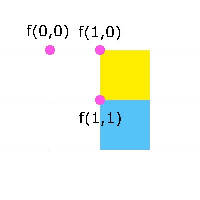
Lets assume we have a line that we want to draw that starts at x0,y0 and ends at x1,y1 we can use the above equation to workout that x0,y0 is on the line because f(x0,y0) = 0 which is no surprise really as its the start of the line. However and here comes the interesting bit, lets say we want to workout the next pixel to draw we have two options. Keep the same y position and just move x by one (yellow) or move both the x and y by one (blue) as shown below
To workout where to draw the next pixel we can plug into the f(x,y) = 0 equation a y of y + 1/2 (a point between are two options) and see if its above or below the line we are trying to draw. If the half way point is below the line we draw the pixel as x + 1, y if it above the line we draw the next pixel as x + 1, y +1.
Using integer Maths the difference approach
Using the half-way (1/2) point is a problem when using integer maths, to get around this the difference approach is used which allows whole numbers to be used. This approach takes the difference between old value x, y (the drawn value) and halfway point x, y + 1/2 of the next point and then makes a decision based off of this difference. For the first difference decision we can use the following equation.
Diff = f(x0 + 1, y0 + 1/2) - f(x0,y0)
Diff = [A(x0 + 1) + B(y0 + 1/2) + C] - [Ax0 + By0 + C]
Diff = [Ax0 + By0 + C + A + 1/2B ] - [Ax0 + By0 + C]
Diff = A + 1/2B
Diff = deltay + 1/2 * -deltax
The decision for the second point (and subsequent points) uses one of the two equations below depending on whether y was increased by one. If y was not increased by one after the first decision the following equation is used.
DiffYsame = f(x0 + 2, y0 + 1/2) - f(x0 + 1, y0 + 1/2) = A = deltay
else this equation is used
DiffYinc = f(x0 + 2, y0 + 3/2) - f(x0 + 1, y0 + 1/2) = A + B = deltay - deltax
For all the difference equations if the difference is positive (point is above the line) the the pixel is drawn at x + 1 , y +1 else the pixel is drawn at x + 1, y (point is below the line). Almost all the half way point testing has been removed using the difference approach this is good for integer maths. However we still use a halfway point test for the first decision, to get around this we can multiply everything by 2. Which will remove the halfway point test at the start but will not affect the signness of the result (ie positive point is still above the line and negative point is still below the line). So we can still make a decision based off of the difference between the two points. So the above equations become
Diff = 2 * deltaY - deltaX
DiffYsame = 2 * deltaY
DiffYinc = 2 * deltaY - 2 * deltaX
Here is the code in chapter 35 that implements the above equations